I had a great discussion recently on the R for Data Science (https://www.rfordatasci.com/ ) Slack channel about how to build a supply chain network model, aligning Customers to Distribution Centers (DC), using the R programming language. Because I am always eager to encourage people new to the supply chain design field, I wrote this small example script. It utilizes ompr for optimization modeling, leaflet for mapping, geosphere for measuring distance, and tidyverse for data prep.
In this example, I use the maps package’s us.cities function, “a database is of us cities of population greater than about 40,000 [and] all state capitals.” Filtering to just Texas, we have a ready-made Customer dataset of 71 cities:
#learning R script on warehouse network design
#install packages if necessary first!
library(tidyverse)
library(magrittr)
library(leaflet)
library(ompr)
library(ompr.roi)
library(ROI.plugin.glpk)

require(geosphere)
require(measurements)
require(maps)

# customer set are the largest cities in Texas

tx_cities <- maps::us.cities %>% dplyr::filter(country.etc=='TX') %>%
  #demand is proportional to population
  dplyr::mutate(demand = ceiling(pop/10))

#real quick leaflet of the cities
leaflet(tx_cities) %>% addTiles() %>% addMarkers()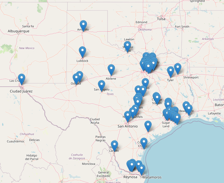
leaflet makes quick mapping a breeze!Now that we’ve used leaflet to verify that all the filtered Customer cities are, in fact, within Texas, we need to create a set of potential warehouse (DC) locations. In most real-life evaluations, you would have more than 6 potential options and they would be created using a combination of qualitative and quantitative techniques. But for this case we’ll just use 6 cities across Texas.
#potential DC sets are Dallas, Amarillo, Houston, El Paso, San Antonio, Beaumont
tx_dc <- tx_cities %>% dplyr::filter(
  name %in% c('Dallas TX','Amarillo TX','Houston TX','El Paso TX',
              'San Antonio TX', 'Beaumont TX'))
In this example, we will require exactly two of these DCs to be opened, without any limitations on either the total number of Customers aligned to each warehouse, nor the total Customer volume aligned to a DC. This is referred to as an unconstrained model. In real life, there are constraints on DC capacity, and those limitations should be built into a real-life network design model.
In unconstrained network design, what you’re trying to do is minimize or maximize the total metric of interest that is incurred by aligning Demand Point D_i to Distribution Center C_j. That metric is usually related to the total network unit-miles. For example, if D_1 has 50 units of demand is aligned to C_2 that is 30 miles away, then the unit-miles are (50*30=1500).
In a warehouse network optimization model, you essentially tell the optimization solver, “here are all the potential combinations, (i * j) options, and here is the metric of interest that matters most to me, and I want you to minimize. Furthermore, here are constraints (restrictions) on those options.”
The optimization solver then finds a solution – a set of Customer / Distribution Center combinations – that either minimizes or maximizes that metric. The metric of interest is often a cost function; in that case, you would tell the solver to minimize. In other cases, the metric may represent a profit function that you would want the solver to maximize. You, as a modeler, input what that metric is. (For those who have a background in optimization modeling or supply chain network design, I know this is a major simplification, but I’m just trying to get across the essence of what optimization modeling does.)
In this example, we will want to minimize the total demand-miles incurred by aligning Customers to DCs. We’ll use the geosphere package to find the pairwise distance, as the crow flies, between each Customer city and potential DC. (This pairwise distance is known as the Haversine distance. The formula is quite complex and takes into account the curvature of the earth; geosphere hides that complex formula behind a function.)
#create a distance matrix between the demand points and DCs
customer_dc_distmat <- geosphere::distm(
  x=cbind(tx_cities$long,tx_cities$lat),
  y=cbind(tx_dc$long,tx_dc$lat)) %>%
  #convert from meters (default) to miles
  measurements::conv_unit('m','mi')
row.names(customer_dc_distmat) = paste0('Customer_',tx_cities$name)
colnames(customer_dc_distmat) = paste0('DC_',tx_dc$name)

#create a matrix that is the metric you wish to minimize or maximize.
#in this example, the metric is unit-miles
#just multiply the demand by city, into the distance from that city to each DC
unitmiles_customer_dc_matrix <-
  tx_cities$demand * customer_dc_distmat


#define scalars for the number of Customers and DC options
customer_count <- nrow(tx_cities)
dc_option_count <- nrow(tx_dc)
Now it’s time to build our optimization model using the ompr package. If you have not had a class in operations research or linear programming, this notation will be new. There are great resources online to learn the basics and I would encourage you to look to find out more.
#now make optimization model
dc_location_model <- ompr::MIPModel() %>%
  #binary decision variables: for each customer, which DC to align to?  Yes/no decisions, align Customer A to DC B yes, or no?
  add_variable(customer_dc_align[customerindex,dcindex],
               customerindex=1:customer_count,
               dcindex=1:dc_option_count,type='binary') %>%
  #binary decision variable: open a DC or no?
  add_variable(open_dc_binary[dcindex],dcindex=1:dc_option_count,type='binary') %>%
  #first constraint: each customer aligned to 1 and only 1 DC
  add_constraint(sum_expr(customer_dc_align[customerindex,dcindex],
                          dcindex=1:dc_option_count)==1,
                 customerindex=1:customer_count) %>%
  #add in "Big M" constraints that activate open_dc_binary when
  #any customers are aligned to a DC
  add_constraint(sum_expr(customer_dc_align[customerindex,dcindex],
                          customerindex=1:customer_count)<=
                   99999*open_dc_binary[dcindex],dcindex=1:dc_option_count) %>%

  #limit the number of opened DCs to EXACTLY 2
  add_constraint(sum_expr(open_dc_binary[dcindex],dcindex=1:dc_option_count)==2) %>%
  #set objective function, the sumproduct
  #of the customer/DC alignment integer variables,
  #and the matrix of the unit-miles for each customer/DC pair
  #sense is either "min" or "max", minimize or maximize the values?
  set_objective(sum_expr(customer_dc_align[customerindex,dcindex]*
                           unitmiles_customer_dc_matrix[customerindex,dcindex],
                         customerindex=1:customer_count,
                         dcindex=1:dc_option_count),sense='min')
With the optimization model built, we now send it to the solver of choice. This code utilizes glpk , but the ompr framework allows for several different linear programming solvers. See https://dirkschumacher.github.io/ompr/ for more.
solution <- ompr::solve_model(dc_location_model,with_ROI(solver = "glpk"))
solution is an object with the overall model solution, including objective function value. We now need to extract the results for the decision variables we care about most: the Customer/DC alignments, customer_dc_align. We’ll then do a little data massaging to bring in the Customer and DC names, latitude, and longitude.
customer_dc_alignment_df <- get_solution(solution,customer_dc_align[customerindex,dcindex]) %>%
  dplyr::filter(value==1) %>%
  dplyr::select(customerindex,dcindex) %>%
  #add in customer and DC names and lat/long
  dplyr::mutate(Customer_City = tx_cities$name[customerindex],
                Customer_Lat = tx_cities$lat[customerindex],
                Customer_Lng = tx_cities$long[customerindex],
                DC_City = tx_dc$name[dcindex],
                DC_Lat = tx_dc$lat[dcindex],
                DC_Lng = tx_dc$long[dcindex]) %>%
  dplyr::select(Customer_City,Customer_Lat,Customer_Lng,
                DC_City,DC_Lat,DC_Lng)
Our only constraints were that each Customer is aligned to a single DC, and there are only two DCs selected. First we’ll check to ensure each Customer City is only present once in customer_dc_alignment_df .
View(table(customer_dc_alignment_df$Customer_City)) #View assumes you're using RStudio.There will be 71 rows in this frequency table, one for each Customer City. Freq values will all be 1, indicating each Customer City is aligned to one and only one DC.
Now verify that only two DCs were selected, Dallas and Houston:
#verify only two DCs selected, should be Dallas and Houston
dc_cities_selected <- unique(customer_dc_alignment_df$DC_City)
dc_cities_selected
[1] "Dallas TX"  "Houston TX"
Now use leaflet to visually inspect the alignments:
#leaflet: color customer city by aligned DC.
customer_dc_alignment_df %<>% dplyr::mutate(
  leaflet_dc_color = dplyr::if_else(DC_City==dc_cities_selected[1],'red','blue'))

leaflet(customer_dc_alignment_df) %>% addTiles() %>%
  addCircleMarkers(lat=~Customer_Lat,lng=~Customer_Lng,
                   color=~leaflet_dc_color,radius=3)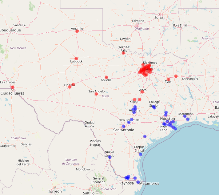
Reassuringly, the cities closer to Dallas, are aligned to the Dallas DC (red dots); and the cities closer to Houston, are aligned to the Houston DC (blue dots). This is in line with our optimization model’s goal of minimizing total unit-miles. The selection of Dallas and Houston as DC locations also makes sense, as they are the anchor cities of Texas’ two largest metropolitan areas, and thus the top two metro areas for demand.
And that’s it! This is a very bare-bones example, but if you’re just starting out, hopefully it will be of help to you! Full code is at https://github.com/datadrivensupplychain/teaching_bits/blob/main/facility_location.r
If you’re interested in learning more about how to improve your supply chain through optimization modeling, simulation, and advanced analytics, please email me ralph@datadrivensupplychain.com to discuss.
Thanks and happy learning!