This is a guest post by Data Driven Supply Chain’s Training Lead, Jeff Clement, PhD
For supply chain management professionals, forecasting is one of the most important – and most frustrating – supply chain planning activities. The forecast is always wrong, the new forecaster hears from their grizzled peer. Yet forecasting, whether it’s of demand, labor, throughput utilization, or more – is fundamental to a smoothly operating supply chain. If you don’t anticipate what’s coming up, how can you prepare?
New and veteran forecasters alike recognize that many products show substantial seasonality, or swings in demand over the course of the year. Demand for ice cream and swimwear is higher in the summer; demand for ski boots and snow sleds is higher in the winter.
This means that just taking last year’s sales and dividing by 12 probably won’t give you a good estimate of a given month’s sales next year. Nor should you necessarily just take last year’s monthly sales, tack on a corporate-approved 3% growth rate, and use that as a forecast.
Seasonality can also be seen at time periods shorter than a year. Brick-and-mortar retail foot traffic, for example, is typically higher on weekends as compared to weekdays, and at certain times of the day. To complicate things even further, seasonality can be highly tied to geography – sales of shorts and t-shirts in Hawaii, with year-round beach weather, is likely more consistent than in icy Minnesota.
Pharmaceutical Demand Data
Let’s load the data we will use for this analysis, looking at the demand for three drugs, aggregated across brands at the monthly level.
The drug demand dataset has three variables:
- Drug: Character; represents the drug
- MonthYear: Date; the last day of the month
- TRX: numeric; the total number of claims for that drug aggregated at the monthly level (rolled up to the last day of the month)
Here’s what the first few rows look like:
| Drug | MonthYear | TRX |
|---|---|---|
| Amoxicillin | 2015-01-31 | 2,631,086 |
| Tacrolimus | 2015-01-31 | 210,607 |
| Dexmethylphenidate | 2015-01-31 | 340,206 |
| Amoxicillin | 2015-02-28 | 2,436,833 |
| Tacrolimus | 2015-02-28 | 194,337 |
| Dexmethylphenidate | 2015-02-28 | 310,181 |
Graph the Time Series
Let’s look at the utilization of these three drugs over time.
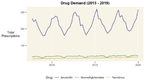
It looks like there is a bit of an upward trend over time, but there are also some seasonal swings. Let’s look at the seasonality using the gg_season command from the feasts package in R.
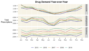
Now we can see things a little more clearly and see that our drugs have wildly different usage patterns.
- Amoxicillin usage doesn’t change too much year-to-year (The lines are fairly close) but there is a big u-shaped utilization pattern over the course of the year. That’s because amoxicillin is an antibiotic used for bacterial infections which peak in winter months and decline in the summer.
- Dexmethylphenidate increases a bit more as time goes on (lines for subsequent years are higher) and there’s a dip in the summer. That’s because dexmethylphenidate is a stimulant used to treat ADHD and for a long time (though they no longer do) the American Academy of Pediatrics recommended children stop taking their ADHD meds in the summer, but some doctors haven’t stopped practicing that way.
- Tacrolimus usage is pretty consistent over the course of the year, but we see big increases (lines jump up from one year to another). That’s because tacrolimus is a daily anti-rejection medication used for organ transplants and there are more people with them every year and they are living longer and longer post-transplant (that’s a good thing!).
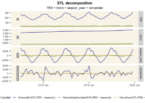
Time series data, including demand data, can be decomposed (separated) into four components: seasonal pattern (regular variation over time), trend (long-term pattern: up, down, or flat), level (long-term average), and any (hopefully small and random) remainder. Performing this STL decomposition helps us better understand demand patterns.
Finally, let’s see how easily we can model and forecast the data.
Modeling and Forecasting
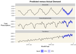
First, let’s exclude the 2019 data and fit a predictive forecasting model on the 2015-2018 data. We’ll use an ARIMA model, which is a type of time series model that can handle both trend and seasonality, and let R fit the best model for us.
Then, let’s forecast the 2019 data and plot the predict the actual vs forecasted data. As you can see, the model does a pretty good job of predicting the future demand for these drugs even without considering any additional variables. These forecasts can then be used for subsequent operational planning.
This is just a quick look at the topic of time series analysis, but even just this quick approach can do a very good job for many applications. If you’re interested in learning more about our training, or how our team can help with demand forecasting, please contact us.