In supply chain management, the newsvendor problem describes an inventory purchasing decision where:
- Inventory is highly perishable (e.g., they can’t be sold tomorrow, like a newspaper)
- Demand is uncertain
- There are costs associated both with overstocking and understocking relative to demand
- There may be a lost sales penalty associated for unmet demand
- There may be salvage values for unsold inventory (e.g., vendor return value, or the tax benefits of inventory markdown)
Many types of products can be modeled with a newsvendor model, pretty much anything that is highly perishable and/or has very little value after a certain date:
- Bakery or dairy foods
- Highly seasonal clothing and decorations (e.g., Halloween costumes)
- Concert tickets
- Nonrefundable airplane tickets
- Physical newspapers / magazines (of course!)
If you have products like this, to determine the optimal (lowest total cost) order quantity you need to determine:
- Cost of Understocking by One Unit: how much money do you give up for each unit of unfulfilled demand? Typically, this is the marginal profit of one unit
- Cost of Understocking Cu = (Cost to Customer) – (Price We Paid) + (Lost Sales Penalty, if any)
- Cost of Overstocking by One Unit: how much money do you give up for each unit of inventory greater than demand? Typically, this is the marginal cost of one unit
- Cost of Overstocking Co = (Price We Paid) – (Salvage Value, if any)
- Probability distribution of demand – assumed to be a normal distribution, a “bell curve”.
- Example: you own a bakery and your daily demand for bearclaw donuts is normally distributed with an average of 50 donuts and a standard deviation of 10 donuts.
- That means that your demand ranges from 40 to 60 donuts, in about 2 out of 3 days; one out of three days, your demand is less than 40 or more than 60.
To calculate the optimal order quantity (the order quantity that maximizes your profit) with the newsvendor model, first calculate the critical ratio, which will be between 0 and 1:
Critical Ratio = Cu / (Cu + Co)
Then find that percentile in the demand distribution of your product, to find the optimal order quantity.
Using our bakery bear claw example
- We estimate that the marginal cost to produce is $0.75
- We sell to customers for $2.00
- Unsold bearclaws can be donated to a food shelf for an estimated $0.25 tax benefit
- We estimate a $0.50 lost sales penalty for unfulfilled demand
So we first calculate the Cost of Understocking by One Unit:
- Cost of Understocking Cu = (Cost to Customer) – (Price We Paid) + (Lost Sales Penalty, if any)
- Cost of Understocking Cu = $2.00 – $0.75 + $0.50 = $1.75
Next we calculate the Cost of Overstocking by One Unit:
- Cost of Overstocking Co = (Price We Paid) – (Salvage Value, if any)
- Cost of Overstocking Co = $0.75 – $0.25 = $0.50
Critical Ratio = Cu / (Cu + Co) = $1.75 / ($1.75 + $0.50) = 0.7778= 77.78%
We now want to find the quantity of bearclaws that will be sufficient to satisfy all demand on 77.78% of days, or 778 out of 1000 days. Remember that our demand is normally distributed with an average of 50 and a standard deviation of 10.
In Excel, the formula NORM.INV(0.7778, 50, 10) gives a result of 57.65 bearclaws to maximize profit, round to 58.
To help drive the point home, I made a web app to demonstrate that the newsvendor problem’s recommended order quantity is, indeed, optimal.
Try out the app here. Adjust input sliders to match your situation. For various order quantities, the app will simulate 50K days of demand and find the average daily profit for each order quantity. Using the bearclaw example, the app looks like this:
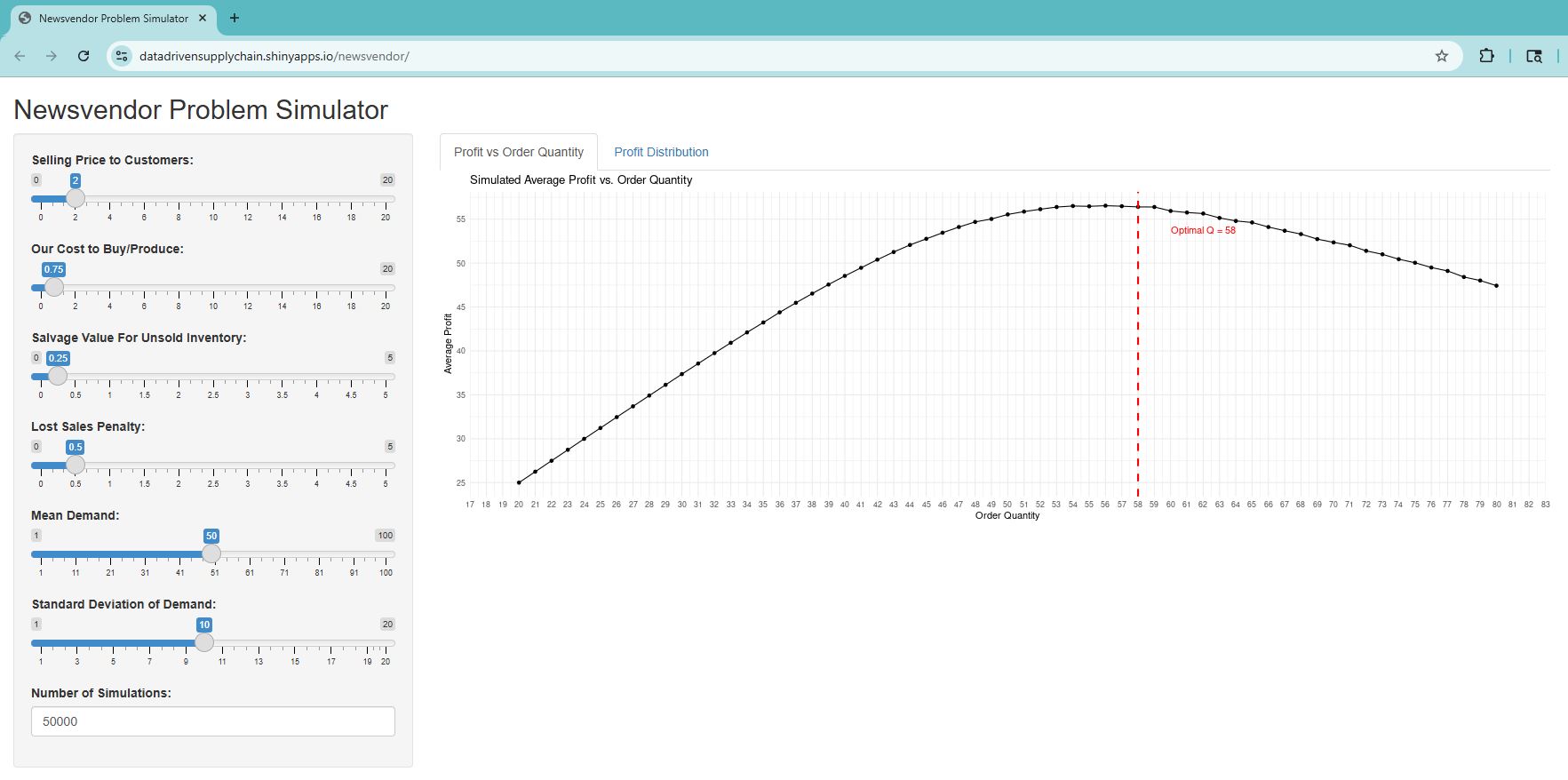
For very low order quantities (e.g., 20 bearclaws), we are almost guaranteed to sell out with an average daily demand of 50. However, we also incur a lot in a lost sales penalties, so the total profit is very low. As we increase the order quantity to 21, 22, and onward, we are still selling out most days, but have fewer lost sales, so the profit increases.
Eventually, around an order quantity of 50 (average daily demand), the profit curve starts to flatten out. As we get past the optimal order quantity of 58, then we have less risk of lost sales – there’s plenty of inventory – but we start to incur the costs of overproduction, so the profit declines.
(Note that because this is a simulation and there is a degree of randomness to it, the profit curves will look slightly different for you. Also, the optimal order quantity of 58 may not have the highest average profit in your simulation – it doesn’t here, either.)
Feel free to play around with this simulation and use it to help your organization!
FYI – At our 2-day training for supply chain data scientists, we cover inventory models including the newsvendor problem, (r,Q) policies, and (s,S) policies.
We recently held this training publicly (recap here), where a satisfied participant said “this may be the best advanced supply chain management data training currently available. I’m grateful to have come. It was well worth the time and investment”.
We offer this training privately for interested organizations. Please reply to discuss.