Note: This content is an introduction to simulation, a powerful tool for analyzing complex supply chain decisions. Simulation allows allows decision-makers to test scenarios, assess risk, and optimize systems without disrupting real operations. To be accessible to a wide audience, this content is not supply chain-specific. However, simulation can be used to improve supply chain applications like Distribution Center operations, inventory management, fleet management and routing, production scheduling, supply chain risk analysis, and much more.
One advantage of entrepreneurship is that while my work hours are long, I can usually work from home, and I have quite a bit of flexibility in when I work. I can take time off in the afternoon to hit the gym or buy some groceries for tonight’s dinner.
I live in the suburbs, so when I go on these small trips, I drive. A while back, I started noticing something strange, going to the gym at a quiet time in the afternoon. I would be sitting in my car, gathering my gym bag. I’d look up and around, and there were so many people right around me, getting in and out of their own cars. Why is that? I’m in a parking lot that easily has 200 cars, and there are maybe ten other people in the lot. So why are five of those ten in my immediate vicinity?
This didn’t happen every time I was at the gym, but it happened enough to notice it more. For a while, I thought it was the Baader-Meinhof Phenomenon; I was just noticing it because it was on my mind. But I saw this happening at the gym. At the pharmacy. At Target. At the grocery store. At McDonalds. (To balance out the gym.) What was going on?
One of the key skills of mathematical modeling (including supply chain modeling) is the ability to look at the complicated real world, identify the core components of a system, and simplify. To figure out what was going on, I simplified the system, and came up with a “model parking lot” for a business. In this model:
- The parking lot has 25 spots, all equally sized and in a single row. The business entrance is at one end. Spaces are designated Space 1 (closest to the business), Space 2 (second closest to the business), … Space 25 (farthest from the business).
- One car arrives in the parking lot every six minutes, starting on the hour (e.g., 8:00 AM, 8:06 AM, 8:12 AM, … 8:42 AM, 8:48 AM, 8:54 AM, 9:00 AM, 9:06 AM …). Thus, ten cars arrive per hour.
- Cars stay in the parking lot exactly thirty minutes: a car that arrives at 8:12 AM will leave at 8:42 AM.
- Cars enter and exit parking spots instantaneously after arriving in the parking lot – no waiting for someone to back out, no waiting in the lane, etc. As such, the parking spot that is vacated at 8:42 AM is immediately available for the car arriving into the lot at 8:42 AM.
- All cars can occupy any open spot – there are no reserved spots, no spots too small for a car, no jerks who apparently don’t know what it means to park between the lines, etc.
- When a car arrives in the parking lot, it immediately occupies the open space that’s closest to the store.
The image below represents the parking lot at 7:59 AM, without any cars in it. The building is assumed to be to the left of Space #1. Space #1 is the closest to the building; Space #25 is the farthest from the building.

Now, anybody can immediately poke holes in this simple model. Cars don’t arrive at nice, even six-minute increments; nor do customers all spend the same amount of time in a business. The idea that you can just immediately vacate or occupy a parking space is laughable. But the laughable simplicity is the point. We start from the simple model and build from there.
Discrete-Event Simulation: What Is It?
It’s a good time to introduce the key analytical method used in this post: discrete-event simulation. Discrete-event simulation (DES) is a powerful way to model systems that operate under uncertainty.
In a discrete-event simulation, you build (in computer code) a model of a system. Systems in DES are, broadly defined, sets of physical and human resources that work together to serve a purpose. Systems can include factories, warehouses, ports, and other facilities in supply chain and logistics; restaurants and stores; websites; call centers; medical facilities… the list is nearly endless.
After building a system in DES, you then subject it to the uncertainties of daily life. “Arrivals” come into the system from outside (deus ex machina) and use resources.
- Customers come into your store
- Trucks arrive at your loading dock for loading or unloading
- Customers arrive at the cashier for checkout
- Cars arrive into the drive-thru at your restaurant
- Patients arrive in the Emergency Department
With DES, you track utilization of resources (e.g., loading docks, X-ray machines, cashiers) over time and make decisions about your business from it. (More accurately, software tracks utilization and you review the results.) Because both the timing and duration of resource usage is highly variable, using simulation allows us to model that uncertainty.
There are many good software options for discrete-event simulation, both open-source and commercial. For this post, and for my consulting work, I use simmer, an excellent R package for discrete-event simulation. I use tidyverse packages for data munging and visualization. If you’re interested in learning how to use simmer, its website has great tutorials; but from this point on, I’ll speak about simulation in a way that is software-agnostic.
In our simplified parking lot example, we are making things easy: there’s no uncertainty. Arrivals occur precisely at 6-minute intervals and leave precisely 30 minutes after arrival. The real world isn’t so nice, but again – we’re intentionally being simplistic to start.
In DES, you (or your software) maintain an event list. The name is descriptive – an event list is simply a way to track changes to the system (“events”) and associate a timestamp with them. While learning about DES in grad school, I had to write out event lists by hand. For demonstration, we’ll do the same here. Using the simplifying assumptions listed above, and assuming the first car arrives at 8:00 AM sharp, we’ll track arrivals, departures, and currently occupied spaces, for a little over an hour.
| Time | Event(s) | Occupied Parking Space(s) |
| 7:59:00 AM | Start of Day | None |
| 8:00:00 AM | Car #1 Arrives, Occupies Space 1 | 1 |
| 8:06:00 AM | Car #2 Arrives, Occupies Space 2 | 1,2 |
| 8:12:00 AM | Car #3 Arrives, Occupies Space 3 | 1,2,3 |
| 8:18:00 AM | Car #4 Arrives, Occupies Space 4 | 1,2,3,4 |
| 8:24:00 AM | Car #5 Arrives, Occupies Space 5 | 1,2,3,4,5 |
| 8:30:00 AM | Car #1 Departs, Opens Up Space 1. Car #6 Arrives, Occupies Space 1. | 1,2,3,4,5 |
| 8:36:00 AM | Car #2 Departs, Opens Up Space 2. Car #7 Arrives, Occupies Space 2. | 1,2,3,4,5 |
| 8:42:00 AM | Car #3 Departs, Opens Up Space 3. Car #8 Arrives, Occupies Space 3. | 1,2,3,4,5 |
| 8:48:00 AM | Car #4 Departs, Opens Up Space 4. Car #9 Arrives, Occupies Space 4. | 1,2,3,4,5 |
| 8:54:00 AM | Car #5 Departs, Opens Up Space 5. Car #10 Arrives, Occupies Space 5. | 1,2,3,4,5 |
| 9:00:00 AM | Car #6 Departs, Opens Up Space 1. Car #11 Arrives, Occupies Space 1. | 1,2,3,4,5 |
| 9:06:00 AM | Car #7 Departs, Opens Up Space 2. Car #12 Arrives, Occupies Space 2. | 1,2,3,4,5 |
The images below represent the progression of the parking lot over the event list. Assuming the building is to the left, space #1 is the far left (closest) space; space #25 is the far right (farthest) space. Green spaces are open; red spaces are occupied. Time progresses from top to bottom, corresponding with the event list we just described.
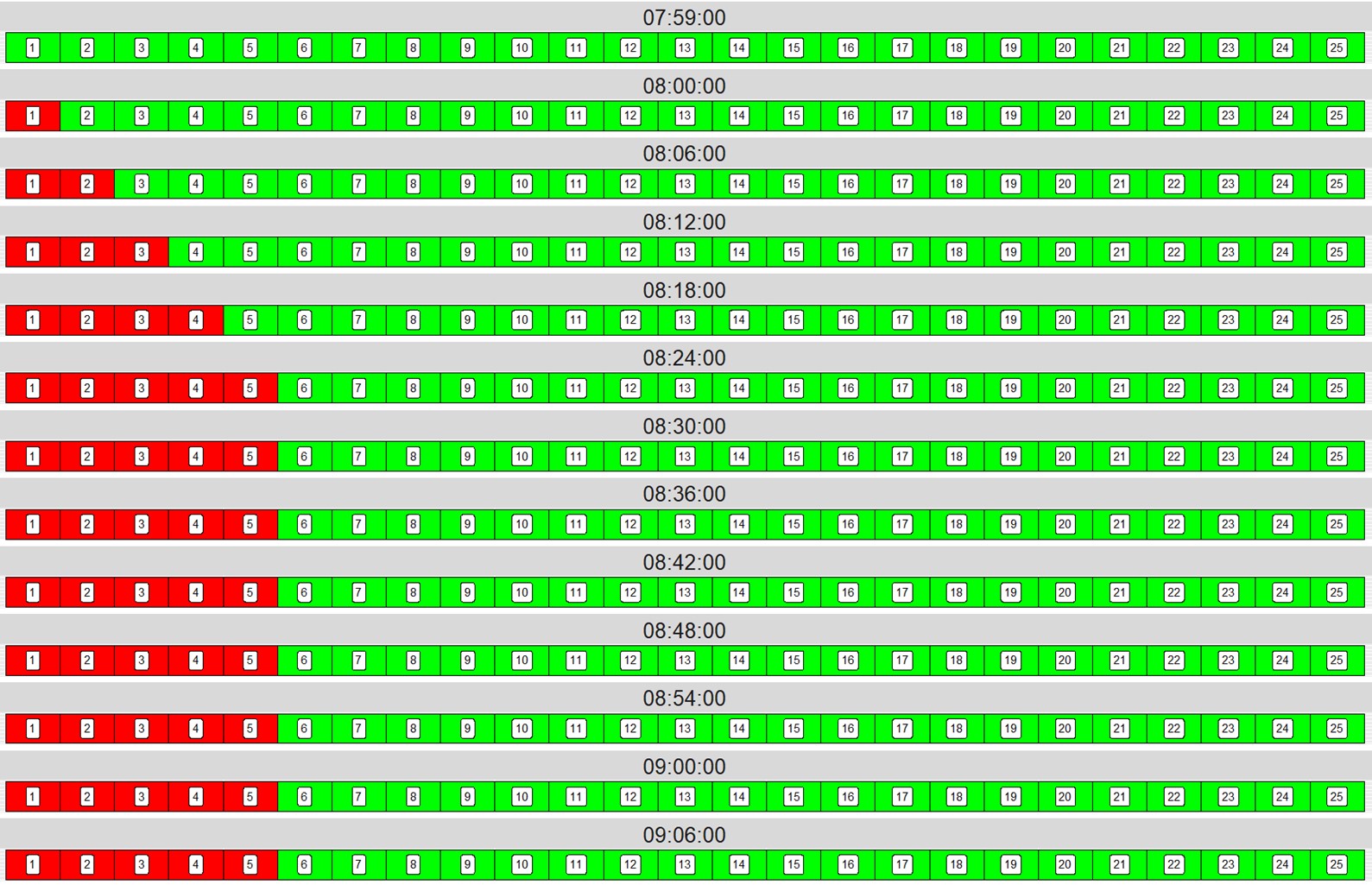
Notice something? Once the fifth car arrives at 8:24 AM, there are five occupied spaces – the five spaces that are closest to the business. And even though cars keep arriving every six minutes, and cars depart after thirty minutes, the occupied parking spaces don’t change. We could keep writing out the event list for hours more – we’d have the same result. This touches on Little’s Law, an important concept in queueing theory, the analytical study of people or things waiting in lines. (Queue being another name for line, uncommonly used in the United States).
Little’s Law, L = Lambda* W, is simple to describe but powerful in application. It applies to any queueing system: pretty much anywhere that people or things arrive, wait for a time, and depart. (Think a parking lot, a loading dock, a restaurant, store, gym, hospital, fill-in-the-blank…)
- L: average number of items in the system. In our example, how many cars, on average, are in the parking lot
- Lambda: average arrival rate into a system. In our example, how many cars enter the parking lot in a specified timeframe: 10 cars arriving every hour, or as an expression: (10 cars / 60 minutes)
- W: average time in the system. In our example, 30 minutes
L = Lambda * W = (10 cars / 60 minutes) * (30 minutes) = 5 cars
Wait! Little’s Law says that on average, we will have 5 cars in the parking lot. After allowing for the first five cars to enter the system, known as a “warm-up period” in simulation studies, this is how many cars (and occupied spaces) we saw when we calculated it by hand. And while we are following the rule that arriving cars take the closest available space, Little’s Law tells us that the 5-car result would occur no matter what spaces were selected.
Where Little’s Law falls short is that the inputs are average rates – not considering variability in those rates.
Ignore Variability At Your Peril
As anybody who has worked the front counter in a retail store or fast-food restaurant can appreciate, these are very different:
- Between 2:00 PM and 3:00 PM, five customers coming in evenly spread out, at 2:00 PM, 2:12 PM, 2:24 PM, 2:36 PM, 2:48 PM. Each require five minutes of attention.
- Between 2:00 PM and 3:00 PM, five customers come in all at once at 2:10PM. Each requires five minutes of attention. No other customers come in until after 3:00 PM.
In both cases, you’re serving five customers in an hour’s stretch – Little’s Law gives the same result for average number of customers in the restaurant. But the impacts on operations, customer satisfaction, and employee stress levels would be very different!
(In college, I worked at a chain sandwich shop that, for legal purposes, I will refer to as Underground Trains. I was, objectively, quite bad at my job as a “Hoagie Designer.” Thank you, Underground Trains, for teaching me real-world lessons on queueing theory.)
Organizations ignore variability at their peril. Looking only at average inputs – customers per hour, truck arrivals per day, production rates per hour – can hide impactful variability in those inputs. That’s one reason why discrete event simulation is so powerful.
Because the world is not as predictable as our initial model of the parking lot, we’re now going to add in some variability to the inputs and see what happens. This table represents the original inputs and assumptions, and any changes we are making to them.
| Initial Modeling Input | Updated Modeling Input |
| The parking lot has 25 spots, all equally sized and in a single row. The business entrance is at one end. | No Change |
| One car arrives in the parking lot every six minutes, starting on the hour. Thus, ten cars arrive per hour. | Cars arrive at an average of 10 per hour, but instead of being uniformly spaced in time, the time between arrivals (“interarrival time”) follow the exponential distribution. The average time between arrivals is still six minutes, but some interarrival times are much shorter than six minutes, and some interarrival times are much longer than six minutes. Another way to say it, arrivals are a Poisson process. |
| Cars stay in the parking lot exactly thirty minutes: a car that arrives at 8:12 AM will leave at 8:42 AM. | The time that cars stay in the parking lot is normally distributed with a mean of 30 minutes and a standard deviation of 5 minutes. |
| Cars enter and exit parking spots instantaneously after arriving in the parking lot | No Change |
| When a car arrives in the parking lot, it immediately occupies the open space that’s closest to the store. | Drivers generally prefer a closer space, but do not always take the closest available. When a car arrives in a parking lot, the open space it occupies is given by the following formula. Suppose there are n open spaces when a car arrives in the parking lot (n ≥1). The open spot closest to the building is designated j =1, the next-closest open spot is designated j = 2, and so on to j = n. A driver will select open spot j with probability 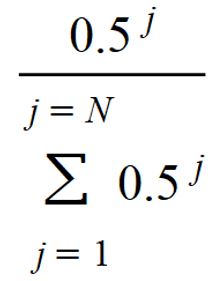 |
| All cars can occupy any open spot | No Change |
You can see how this may change how our parking lot looks over time. Arrivals are not as predictable; how long a car stays in the parking lot is not as predictable; where they park is not as predictable. Thankfully, discrete-event simulation allows us to, relatively quickly, simulate the parking lot under this uncertainty. DES software randomly generates cars’ arrival times and length of time in the parking lot, based upon the parameters we set. DES software then tracks the status of each parking space (and the lot as a whole) as the day progresses. Below, we see the status of the parking lot in one simulation, with an average of 10 arrivals per hour, and an average of 30 minutes parked. In this visual, we’re looking at the parking lot every 20 minutes, from 8:00 AM to 12:00 PM (noon).
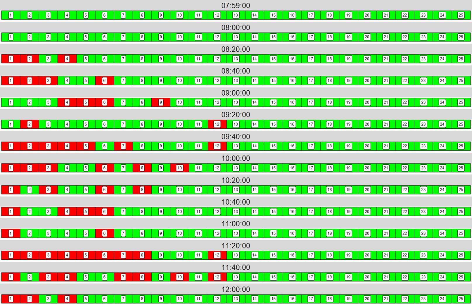
Not so predictable, is it! Over the course of an entire day, the average number of cars in the lot is still (very close) to 5, in accordance with Little’s Law. (Trust me for now on this one). But the variability is significant. At 8:20 AM, only three cars are in the lot. At 11:20 AM, nine cars are.
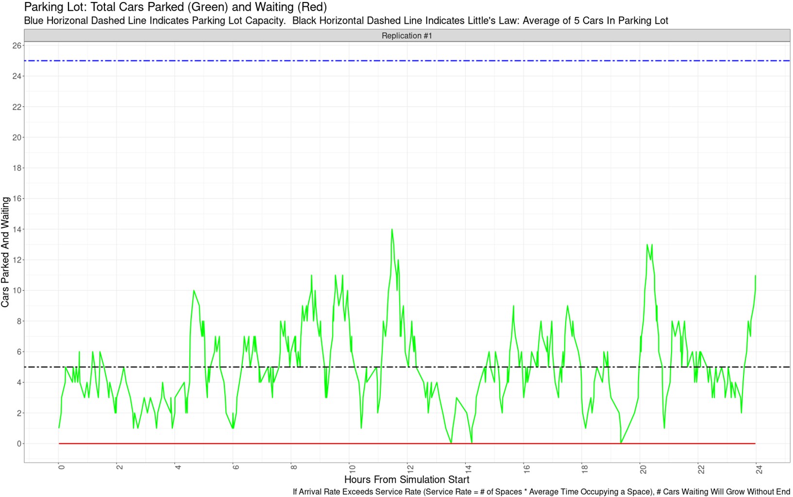
If we were to track the number of cars in the lot over 24 hours, it may look like the following plot. The x-axis is hours since the simulation started (so x=0 refers to 8:00 AM, x=2.5 refers to 10:30 AM, and so forth). The y-axis represents the number of cars parked (green line) and waiting to park, if any (red line, zero throughout the simulation). You can see that while the number of parked cars is approximately balanced around 5, as Little’s Law suggests, there is significant variability throughout the day.
You may be thinking at this point, “But wait! If the cars’ arrival times are no longer predictable, and the time that a car spends in the parking space is no longer predictable, how useful is tracking the number of cars in the lot? Won’t it be variable, just like the inputs are variable?”
If you are thinking that: the answer is YES! (Also, you possibly know a bit about simulation.) In discrete-event simulation, you have two sides of the coin: you can incorporate the randomness of real life, but your results are dependent on the specific randomness you include!
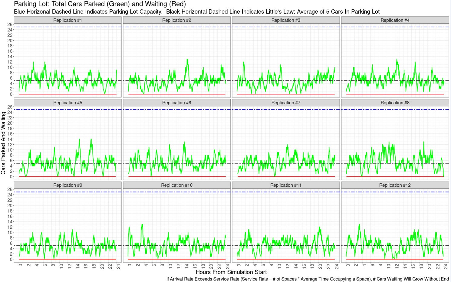
The impact of this randomness can be mitigated by replicating the simulation multiple times and aggregating the results for analysis. If we replicated the parking lot simulation twelve times and plotted the time series of the number of cars in the lot for each replication, it may look like the image below. You can examine each time series and see that there are differences between replications. But in each replication, the average number of cars in the lot (over time) is very close to 5, as Little’s Law would suggest. (Note, the time series above is not represented in the replications below).
If you run multiple replications of a simulation, you can track utilization of a resource (the whole parking lot, or an individual space) over time. You can also find the resource’s total utilization over the course of a replication, then create a boxplot that aggregates each resource’s utilization across replications.
The image below is such a boxplot, showing aggregated utilization across the twelve replications that generated the time series plot above. The boxplot indicates minimum, maximum, median, and interquartile range (IQR) of utilization. A red dot indicates average (mean) utilization.
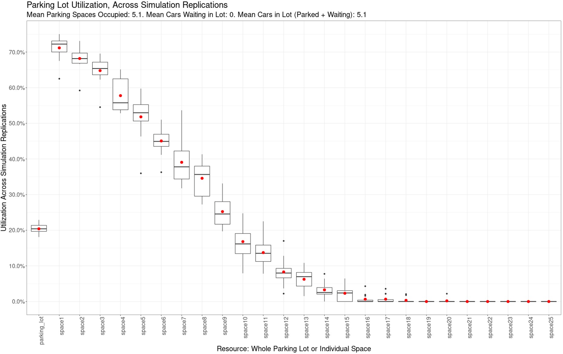
On the far left of the x-axis, we see the utilization of the whole parking lot. Its utilization across replications is quite similar, with a mean and median utilization just above 20%. With a capacity of 25 spaces, and a utilization of 20%, the parking lot contains, on average, (25 * 20%) = 5 cars, as Little’s Law suggests. (The subtitle states that the actual mean is 5.1 cars – simulation results do not always match theory exactly.)
On the x-axis, after the whole parking lot, the axis proceeds left-to-right with the utilization of individual spaces. Remember that space1 denotes the parking space closest to the building; space2 denotes the next-closest parking space; and space25 denotes the space furthest from the building.
Because drivers generally prefer to park closer to the building, utilization for space1 – the space closest to the building – is consistently high, and averages around 71%. Utilization gradually drops the further away from the building you get, and spaces 14 through 25 are barely used, if at all. (Next time you’re at a big-box store and the lot isn’t full, see how many of the far back spaces are used. Not many, I’d guess.)
I’ve developed an app that allows you to experiment with the input parameters and see how it changes the parking lot’s utilization (the app’s output is very similar to the previous two images). You can also see what happens when each open parking spot has an equal probability of selection, and what happens when the expected number of cars in the system, per Little’s Law, is greater than the number of parking spaces. (Hint: lots of waiting, and an ever-growing number of cars circling the parking lot in vain.)
Please note that it may take some time to run the simulation in the app. You’ll receive a popup notification when outputs are ready to view.
Conclusion… So Why Are So Many People Near My Car?
Now, it’s time to answer the original question that prompted this post. When I’m entering or leaving a spot in a parking lot, why does it seem like so much activity is occurring right around me?
To answer this, we again first make a simplistic model. Assuming a parking lot that is 25 spaces in a single row, we can find the distance between each pair of spaces. For example, the distance between Space #1 to Space #3 is two spaces; the distance between Space #16 and Space #25 is nine spaces. We can then make a histogram of the pairwise distances between all spaces.
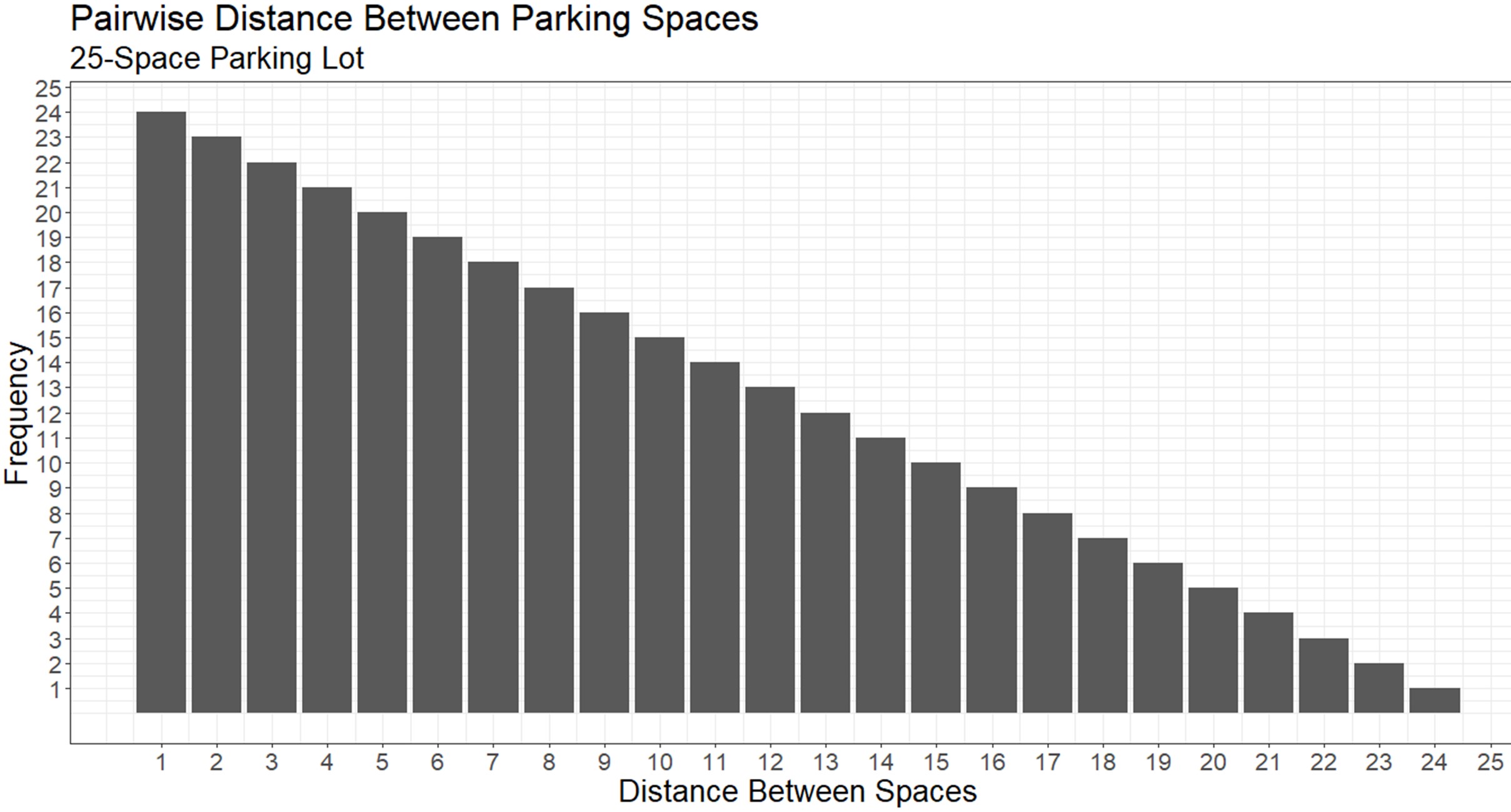
The least common distance was…24 spaces. This makes sense when you stop to think about it a bit. There is only one pair of spaces that are exactly 24 spaces apart: #1 and #25. The next least-common distance was 23 spaces. There are only two pairs of spaces that are exactly 23 spaces apart: #1 & #24, and #2 and #25. You can continue this logic all the way from right to left on the chart, until we get to the most common distance between a pair of spaces: one space. (#1 & #2, #2 & #3, and so on until we get to #24 & #25. Twenty-four occasions in all.)
This is an interesting starting point, because it suggests that if we pick two spaces at random, the most common distance between them is 1, with an 8% probability. There would be a 37% probability of them being five or fewer spaces apart, with an average distance of 8.667 spaces.
You can test this yourself with a computer program, or more analog, you can perform an experiment using ping pong balls or slips of paper marked #1 through #25.
This effect is likely to be more pronounced in our parking lot simulation. Remember, people tend to park as close to the building as possible, and the farther-away spots are rarely used, at least in lower-traffic times. In the utilization boxplot above, look at the utilization of spaces #12 through #25: minimal. This suggests that simultaneous arrivals/departures are much more likely to occur in spaces that are near each other, because we’re all just trying to park in the front of the parking lot.
To measure this effect in the parking lot simulation is a little more complex, but just a little. The simmer package in R provides detailed simulation output in data frames, including arrival and departure times for each car and parking space. From that, you can identify:
- When arrivals/departures occur within a specified time window of each other. In this example, I am calling any pair of arrivals or departures that occur within 5 minutes of each other, “near-simultaneous.”
- How many pairs of arrivals or departures are “near-simultaneous.”
- Out of those pairs that are near-simultaneous, how many parking spaces apart were they?
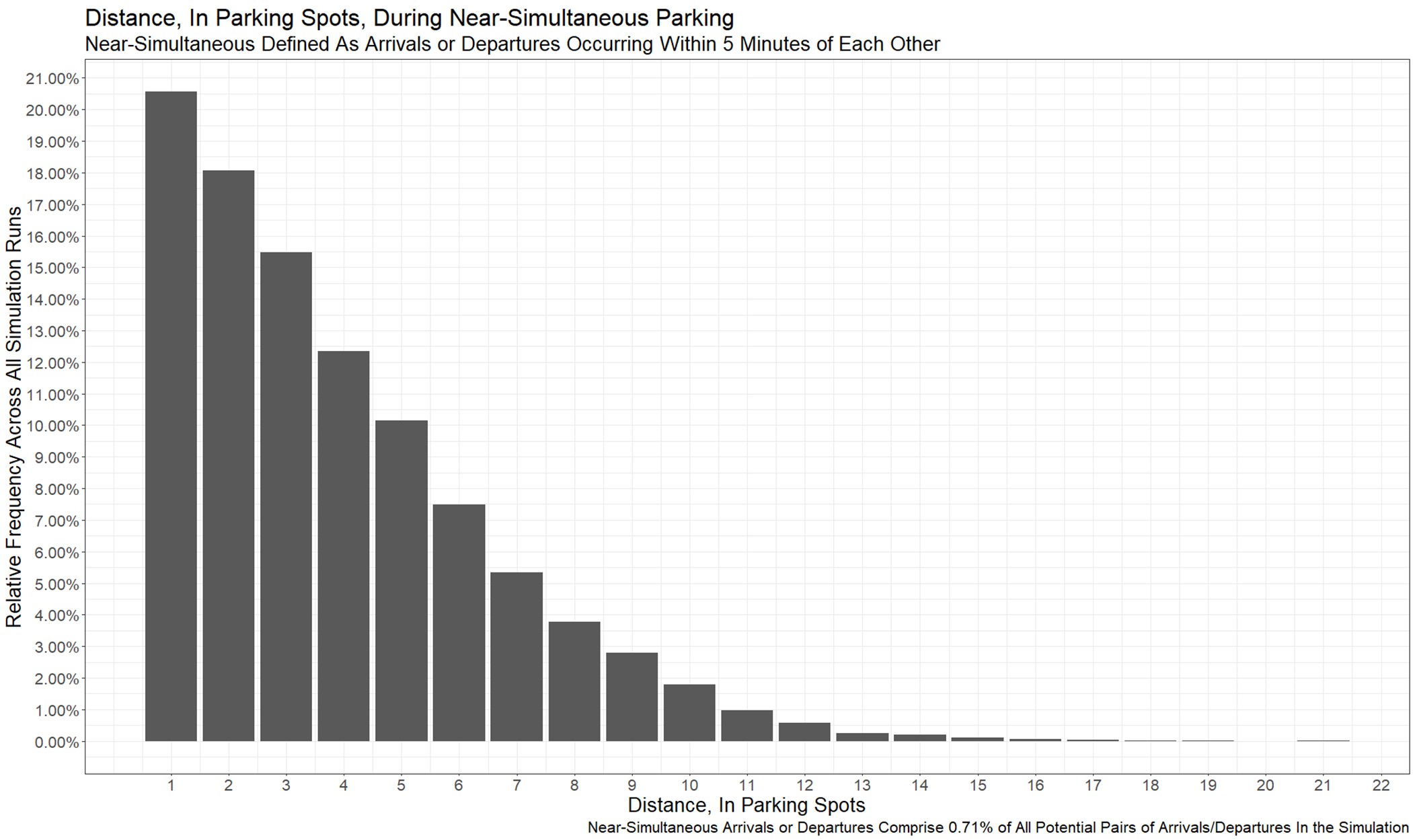
The following plot shows the result. Out of all arrival/departure pairs in the simulation, less than 1% occurred within 5 minutes of each other. (Given that these simulations represent 24 hours of simulated time, that’s not too surprising.) But out of the “near-simultaneous” arrivals & departures, over 20% were in adjacent spaces (distance = 1 on the x-axis). Just over half were three or fewer spaces apart – pretty close, as far as parking lots go.
So why are so many people parking right around me at the gym? Statistics and probability, folks. That’s why. Also, because I don’t want to walk further than absolutely necessary to get to the treadmills.
(Note that this bar plot would look pretty much the same if we defined “near-simultaneous” as occurring within five minutes, ten minutes, or 12 hours of each other… the relative frequency percentages would be quite stable.)
Real Conclusion
I hope you have found this post entertaining and informative about the power of discrete-event simulation (DES). Alas, I’ve only scratched the surface of the power of DES. With DES, you can model complex, multi-staged processes like manufacturing plants, warehouses, and logistics hubs. Using DES, you can understand the impact of significant changes to business processes before engaging in costly and hard-to-correct capital projects. Using DES, you can understand how to plan for extreme swings in your business, like if your manufacturing plant had to increase production by 25% overnight, or if your store’s weekly traffic doubled from this week to next.
Data Driven Supply Chain LLC offers consulting services and training at the intersection of data science and supply chain. Please reach out using the contact form below to learn more about how simulation, and other techniques from data science, can be used to evaluate, improve, and design your supply chain.
Thank you for reading, and happy simulating!
Updated April 17, 2025